558Basic
Cosmetic API Vignette
Vivi Feathers 2023-10-03
This document is a vignette with the purpose of exploring how to read in data using a function created for interacting with a specific API, as well as showing different types of data analyses that can be conducted on the data obtained.
I’ll be demonstrating with the MAKEUP API which contains cosmetic items’ name, brand, type, price and rating. I’m going to build a few functions to interact with 2 endpoints: product brand and product type.
I will also summarize the statistics of price and rating by product type with all the data available. After data are fetched and cleaned based on the brand and/or type selected, I will merge the summaries with the fetched data and compare each item’s price and rating verse price and rating summaries from the corresponding product type, thus the user may have some ideas about whether to choose this item or not.
The second part of the vignette focus on data exploration, I will investigate cosmetic items’ brand, type, price and rating by creating some contingency tables, numerical summaries and couple of plots.
Requirement
The following packages were used to create this document:
tidyverse: used for data manipulation, piping and visualizationjsonlite: used for interacting with JSON in the API and returning data in data frameknitr: used to manage code in R Markdown format
API Interaction Functions
clean_data
I created a data cleaning function that removes confusing columns and keep brand, name, product_type, price, currency, rating, description, image_link columns. It also omits records with missing price or “0.0” as price value, and removes carriage returns from the name and description column. Additionally, it converts price to numeric values, rounds them to two decimal places and standardizes them as US dollars according to their currency name (CAD x 0.73, GBP x 1.22, if currency is missing, I take it as USD by default).
# create a data cleaning function that removes confusing columns, keep records with non-missing price,
# removes carriage returns,converts price to numeric values, standardized them as US dollars according to
# currency name.

clean_data <- function(df){
    df%>%
      select(brand, name, product_type, price, currency, rating, description, image_link) %>%
      filter (is.na(price) == FALSE & price != "0.0") %>%
      mutate(description = gsub("[\r\n]", "", description),
             name = gsub("[\r\n]", "", name),
             usd_price = if_else(is.na(currency) == TRUE, round(as.numeric(price)*1, digits =2),
                                 if_else(currency == "GBP", round(as.numeric(price)*1.22, digits =2),
                                         if_else(currency == "USD", round(as.numeric(price)*1, digits =2),
                                                 if_else(currency == "CAD", round(as.numeric(price)*0.73, digits =2), 0)))))
  }
price_sum and rating_sum
I grabbed all the available data by calling the base URL in fromJSON
function. After cleaned the raw “all_type” data frame by using the
“clean_data” function. I summarized the price statistics (mean, median,
25th and 75th percentile) across product type. Then I removed the
records with missing rating, and calculated the rating statistics (mean,
median, 25th and 75th percentile) by product type as well, At the end, I
stored the results into two data frames: price_sum and rating_sum.
# use `fromJSON` function to get data frame from the base url and name it as "all_type"

all_type <- fromJSON("http://makeup-api.herokuapp.com/api/v1/products.json?")

# clean the raw "all_type" data frame by calling the "clean_data" function

all_type_clean <- clean_data(all_type)

#calculate the price statistics (mean, median, 25th and 75th percentile)

price_sum <- all_type_clean %>%
               group_by(product_type) %>%
               summarise(type_price_avg = mean(usd_price),
                         type_price_q1 = quantile(usd_price, probs = 0.25),
                         type_price_q3 = quantile(usd_price, probs = 0.75),
                         type_price_median = median(usd_price))

# remove the missing values from rating and calculate the rating statistics

rating_sum <- all_type_clean %>%
                filter(is.na(all_type_clean$rating) == FALSE) %>%
                group_by(product_type) %>%
                summarise(type_rate_avg = mean(rating),
                          type_rate_q1 = quantile(rating, probs = 0.25),
                          type_rate_q3 = quantile(rating, probs = 0.75),
                          type_rate_median = median(rating))
pick_makeup
I created an API interaction function that fetches data based on user selected cosmetic brand or/and product type.
Step one, I set up the base URL which returns all the available data; I also defined the brand pool and the type pool to limit user’s selections in “benefit”, “dior”, “covergirl”, “maybelline”, “smashbox”, “nyx”, “clinique” as cosmetic brands and “lipstick”, “foundation”, “eyeliner”, “eyeshadow”, “mascara”, “blush” as product types.
Step two, I checked the user’s argument input values to make sure both “makeup_brand” and “makeup_type” are character strings that within the brand and type pool, otherwise the function will stop executing. After making sure the input values are good, I paste them with the base URL to form the API with endpoints.
Step three, I used fromJSON function to obtain a data frame from the
“api_url” and name it as “target”.
Step four, I cleaned the raw “target” data frame by calling the “clean_data” helper function, and stored the processed data frame in “target_clean”.
Step five, I merged price and rating summaries from “price_sum” and “rating_sum” data frames with “target_clean” data frame by product type.
Step six, I compared the price and rating of each observation from the “target_clean” data frame vs the corresponding price summary and rating summary from the same type products, and return “higher than”, “equal to” and “less than” accordingly.
Step seven, I pasted the item price, product type, price/rating summary and comparison results from step six together and output them into “price_stat” and “rating_stat” column as price and rating status for each observation.
Lastly, I returned the final data frame by keeping the necessary columns as brand, name, product_type, usd_price, price_stat, rating, rating_stat, description and image_link.
pick_makeup <- function(makeup_brand = NULL, makeup_type = NULL){

  # set up the base URL
  api_url <- "http://makeup-api.herokuapp.com/api/v1/products.json?"

  #set up brand and type option pool
  brand_base <- c("benefit", "dior", "covergirl", "maybelline", "smashbox", "nyx", "clinique")
  type_base <- c("lipstick", "foundation", "eyeliner", "eyeshadow", "mascara", "blush")

  # check the input values
  if (!is.null(makeup_brand)){
    # makeup brand must be a characters string, if not, stop the function and return message.
    if (!is.character(makeup_brand)){
      stop("makeup brand must be a character string.")
    }
    # makeup brand must be selected from the brand pool, if not, stop the function and return message.
    makeup_brand <- tolower(makeup_brand)
    if (! (makeup_brand %in% brand_base)){
      stop("makeup brand must be selected from benefit, dior, covergirl, maybelline, smashbox, nyx and clinique.")
    }
    # if makeup_brand is not missing, it is a character string that from the brand pool, paste it into base url.
    api_url <- paste0(api_url, "brand=", makeup_brand)
  } # if makeup_brand is missing, leave "brand=" piece empty in the url
  else{api_url <- paste0(api_url, "brand=")}

  if (!is.null(makeup_type)){
    # makeup type must be a characters string, if not, stop the function and return message.
    if (!is.character(makeup_type)){
      stop("makeup type must be a character string.")
    }
    # makeup type must be selected from the type pool, if not, stop the function and return message.
    makeup_type <- tolower(makeup_type)
    if (! (makeup_type %in% type_base)){
      stop("makeup type must be selected from lipstick, foundation, eyeliner, eyeshadow, mascara, blush.")
    }
    # if makeup_type is not missing, it is a character string that from the type pool, paste it into base url.
    api_url <- paste0(api_url, "&product_type=", makeup_type)
  }# if makeup_type is missing, the "api_url" remains unchanged

  # use `fromJSON` function to get data frame from the "api_url" we just set up and name it as "target"
  target <- fromJSON(api_url)

  # clean the raw "target" data frame by calling the "clean_data" function
  target_clean <- clean_data(target)

  # merge price and rating summaries with target data frame by product type and do the comparison

  target_price <- merge(target_clean, price_sum, by="product_type")
  target_price_rate <- merge( target_price, rating_sum, by="product_type")

  # compared the price and rating of each observation vs summaries from the same type products

  target2 <-  target_price_rate %>%
    mutate(comp_mean = if_else(usd_price > type_price_avg, "higher than",
                               if_else(usd_price < type_price_avg, "lower than",
                                       if_else(usd_price == type_price_avg, "equal to", ""))),
           comp_median = if_else(usd_price > type_price_median, "higher than",
                                 if_else(usd_price < type_price_median, "lower than",
                                         if_else(usd_price == type_price_median, "equal to", ""))),
           comp_q1 = if_else(usd_price > type_price_q1, "higher than",
                             if_else(usd_price < type_price_q1, "lower than",
                                     if_else(usd_price == type_price_q1, "equal to", ""))),
           comp_q3 = if_else(usd_price > type_price_q3, "higher than",
                             if_else(usd_price < type_price_q3, "lower than",
                                     if_else(usd_price == type_price_q3, "equal to", ""))),
           comp_rt_mean =  if_else(as.numeric(rating) > type_rate_avg, "higher than",
                                   if_else(as.numeric(rating) < type_rate_avg, "lower than",
                                           if_else(as.numeric(rating) == type_rate_avg, "equal to", ""))),
           comp_rt_median = if_else(as.numeric(rating) > type_rate_median, "higher than",
                                    if_else(as.numeric(rating) < type_rate_median, "lower than",
                                            if_else(as.numeric(rating) == type_rate_median, "equal to", ""))),
           comp_rt_q1 = if_else(as.numeric(rating) > type_rate_q1, "higher than",
                                if_else(as.numeric(rating) < type_rate_q1, "lower than",
                                        if_else(as.numeric(rating) == type_rate_q1, "equal to", ""))),
           comp_rt_q3 = if_else(as.numeric(rating) > type_rate_q3, "higher than",
                                if_else(as.numeric(rating) < type_rate_q3, "lower than",
                                        if_else(as.numeric(rating) == type_rate_q3, "equal to", ""))))

  # generate "price_stat" and "rating_stat" column by pasting the item price, product type, price/rating summary and comparison results

  target3 <- target2 %>%
    mutate(price_stat = paste0("This ", product_type, "'s price is $", usd_price, " which is ", comp_mean,
                               " the overall ", product_type, " price mean (", round(type_price_avg, digits=2), "), ", comp_median,
                               " the price median(", round(type_price_median, digits=2),"), ", comp_q1,
                               " the 25th percentile(", round(type_price_q1, digits=2),"), and ", comp_q3,
                               " the 75th percentile(", round(type_price_q3, digits=2),")."),
           rating_stat = if_else(is.na(rating)==TRUE, "No rating",
                                 paste0("This ", product_type, "'s rating is ", rating, " which is ", comp_rt_mean,
                                        " the overall ", product_type, " rating mean (", round(type_rate_avg, digits=2), "), ", comp_rt_median,
                                        " the rating median(", round(type_rate_median, digits=2),"), ", comp_rt_q1,
                                        " the 25th percentile(", round(type_rate_q1, digits=2),"), and ", comp_rt_q3,
                                        " the 75th percentile(", round(type_rate_q3, digits=2),").")))
  # keep necessary columns and return
  target_final <- target3 %>%
    select(brand, name, product_type, usd_price, price_stat, rating, rating_stat, description, image_link)
  return(target_final)
}
Exploratory Data Analysis (EDA)
Now the API interaction function is done, I can explore some data analysis.
First call
First of all, let’s call the API function with default argument inputs
and return all the available data, then write a function add_factor
which converts cosmetic brand and product type as factors, that way it
will be better for data analysis.
# call the function and return all the data
all <- pick_makeup(makeup_brand = NULL, makeup_type = NULL)

# write a function to convert "brand" and "product_type" to factors
add_factor <- function(df_1) {
                    df_1 %>%
                       mutate(Cosmetic_Brand = as.factor(df_1$brand), Cosmetic_Type = as.factor(df_1$product_type))
}

all_factor <- add_factor(all)
Two-way contingency table
Let’s use a table function and create a two-way contingency table and
break the item counts by brand and type.
two_way <- table( all_factor$Cosmetic_Type,all_factor$Cosmetic_Brand)
two_way
##
##               almay alva anna sui annabelle benefit boosh burt's bees butter london cargo cosmetics china glaze
##   blush           1    0        1         1       0     0           0             0               3           0
##   bronzer         1    0        0         1       6     0           0             0               9           0
##   eyeliner        3    0        3         7       3     0           0             0               2           0
##   eyeshadow       2    1        0         0       0     0           0             0               1           0
##   foundation      3    0        0         1       2     0           0             0               2           0
##   lip_liner       0    0        0         1       0     0           0             0               1           0
##   lipstick        1    0        1         0      13     1           2             1               2           0
##   mascara         3    0        0         0       6     0           0             0               0           0
##   nail_polish     0    0        1         0       0     0           0             1               0           1
##
##               clinique colourpop covergirl dalish deciem dior dr. hauschka e.l.f. essie fenty glossier l'oreal
##   blush              7         0         7      0      0    4            0      2     0     0        1       2
##   bronzer            5         0         2      0      0    1            3      5     0     0        0       1
##   eyeliner           9         0        12      0      0    6            2      4     0     1        0       9
##   eyeshadow         12         0         5      0      0   10            2      6     0     0        0       1
##   foundation        34         1        10      0      2    9            2      3     0     2        4       7
##   lip_liner          2         1         1      0      0    0            0      1     0     0        0       2
##   lipstick          17         2         4      1      0   15            2      3     0     2        1       7
##   mascara            0         0        12      0      0    8            1      3     0     0        0       8
##   nail_polish        0         0         1      0      0   13            0      0     4     0        0       9
##
##               marcelle maybelline milani mineral fusion misa mistura moov nyx orly pacifica physicians formula
##   blush              1          4      2              1    0       0    0  12    0        1                  8
##   bronzer            2          3      1              1    0       0    0   9    0        1                  9
##   eyeliner           4          8      5              1    0       0    0  32    0        1                  9
##   eyeshadow          1          7      1              0    0       1    0   1    0        4                  3
##   foundation         2         10      1              2    0       0    0  32    0        0                  8
##   lip_liner          3          1      1              0    0       0    0  10    0        1                  0
##   lipstick           1          7      2              1    0       0    0  38    0        1                  0
##   mascara            1         11      0              1    0       0    0  11    0        2                  6
##   nail_polish        0          3      0              1    1       0    3   0    4        2                  0
##
##               piggy paint pure anada revlon salon perfect sante sinful colours smashbox stila suncoat wet n wild
##   blush                 0          3      2             0     1              0        3     2       0          0
##   bronzer               0          1      0             0     0              0        2     1       0          0
##   eyeliner              0          1      4             0     1              0        6     1       1          5
##   eyeshadow             0          2      1             0     1              0        7     0       0          3
##   foundation            0          4      7             0     1              0        9     0       0          0
##   lip_liner             0          0      1             0     1              0        0     0       0          0
##   lipstick              0          1     11             0     0              0        6     0       0          2
##   mascara               0          1      0             0     0              0        6     0       1          1
##   nail_polish           1          3      3             1     1              1        0     0       4          1
##
##               zorah
##   blush           0
##   bronzer         0
##   eyeliner        1
##   eyeshadow       0
##   foundation      0
##   lip_liner       0
##   lipstick        0
##   mascara         1
##   nail_polish     0
The two-way contingency tables shows that there are 44 cosmetic brands and 9 product types. “covergirl”, “l’oreal” and “maybelline” are the only 3 brands have products in all 9 types. “alva”, “boosh”, “burt’s bees”, “china glaze”, “dalish”, “deciem”, “essie”, “misa”, “mistura”, “moov”, “orly”, “piggy paint”, “salon perfect” and “sinful colours” only have one type products in the database. “nyx” has the most items and “alva”, “boosh”, “china glaze”, “dalish”, “misa”, “mistura”, “piggy paint”, “salon perfect” and “sinful colours” only have one item.
Stacked bar graph
I want to know the item count by product type. I will use gglot and
geom_bar to create a stacked bar graph to present item count for each
product type with cosmetic_type as x, also fill colors based on
different product type.
g <- ggplot(data = all_factor, aes(x = Cosmetic_Type, fill = Cosmetic_Type))
g + geom_bar(alpha = 0.6) +
  labs(x = "Cosmetic Type", y = "Item count", title = "Bar Plot of Item Count for Each Cosmetic Type")
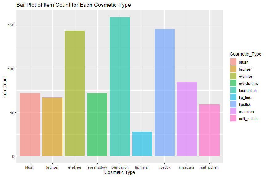
From the bar plot we can see, the blush, bronzer, eyeshadow, mascara and nail polish product types each has around 60 to 80 items, the eyeliner and the lipstick categories have around 140 item each. The foundation category has the most items and the lip liner has the least products.
Price summary by cosmetic type.
In order to know more about price, I will calculate the price mean,
standard deviation, variance, median, Q1 and Q3 across product types by
using a group_by and a summarise function.
all_factor %>%
  group_by(Cosmetic_Type) %>%
  summarise(Mean = mean(usd_price),  Standard_Deviation = sd(usd_price),
            Variance = var(usd_price), Median = median(usd_price),
            q1 = quantile(usd_price, probs = 0.25),
            q3 = quantile(usd_price, probs = 0.75))
## # A tibble: 9 × 7
##   Cosmetic_Type  Mean Standard_Deviation Variance Median    q1    q3
##   <fct>         <dbl>              <dbl>    <dbl>  <dbl> <dbl> <dbl>
## 1 blush          18.5              10.8     117.   15.2   9.99  24.1
## 2 bronzer        23.5              13.9     194.   21.0  11.2   32
## 3 eyeliner       13.2               6.88     47.4  11     8     17.0
## 4 eyeshadow      22.2              16.3     267.   17.7   9.98  28
## 5 foundation     21.4              11.4     129.   20.0  12     28
## 6 lip_liner      10.2               5.16     26.6   9.99  4.99  13.0
## 7 lipstick       15.9              11.0     121.   12     8     21
## 8 mascara        15.4               8.54     72.9  13.0   9     22
## 9 nail_polish    14.1               7.25     52.6  11.0   8.14  22.2
From this summary table we can tell that the data distribution of almost all product types are skewed. The data distribution of lip liner category is the closest to normal distribution compared with other product types. Bronze category has the highest mean and median, eyeshadow category has the widest variance while lip liner category has the lowest mean, median and narrowest variance.
Violin plot
I am curious about rating distribution. Because lots of cosmetic
products have missing ratings, let’s choose five brands which have the
least missing rating values, and use gglot and geom_violin to create
violin graph for their rating distributions. I will map cosmetic_brand
as x, rating as y also fill the violins with customized colors based on
different cosmetic brand.
#filter to 5 brands that have most non-missing rating
five_brand <- all_factor %>%
              filter(Cosmetic_Brand %in% c("l'oreal", "physicians formula", "covergirl", "maybelline", "revlon"))

p <- ggplot(data = five_brand, aes(x = Cosmetic_Brand, y = rating, fill = Cosmetic_Brand))
p + geom_violin(alpha = 0.6) +
scale_fill_manual(values=c("#EF6F6A", "#cc9900", "#69b3a2", "#404080", "#9172EC")) +
labs(x = "Cosmetic Brand", y = "Rating Distribution", title = "Violin Plot of rating distribution across cosmetic brands")
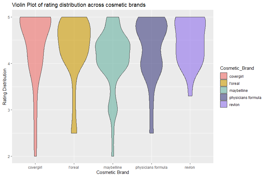
Almost all distributions are left-skewed, meaning most rating are at the high end. Overall, “revlon” has the best rating since all of its rating are above 3.3; “maybelline” has the worst rating because most of its rating are below 4.5, only a small portion reached 5. It follows a multimodal distribution with a big peak at 4.3 and a small peak at 3. “physicians formula” also follows a multimodel distribution with two peaks at 4.8 and 4.
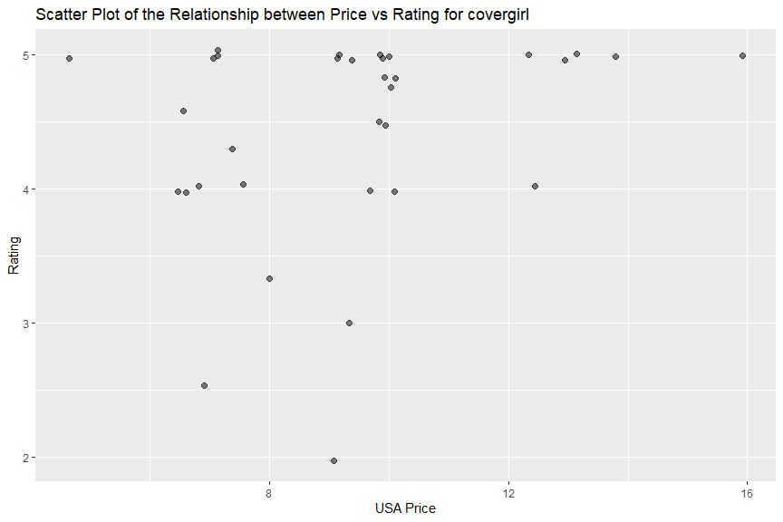
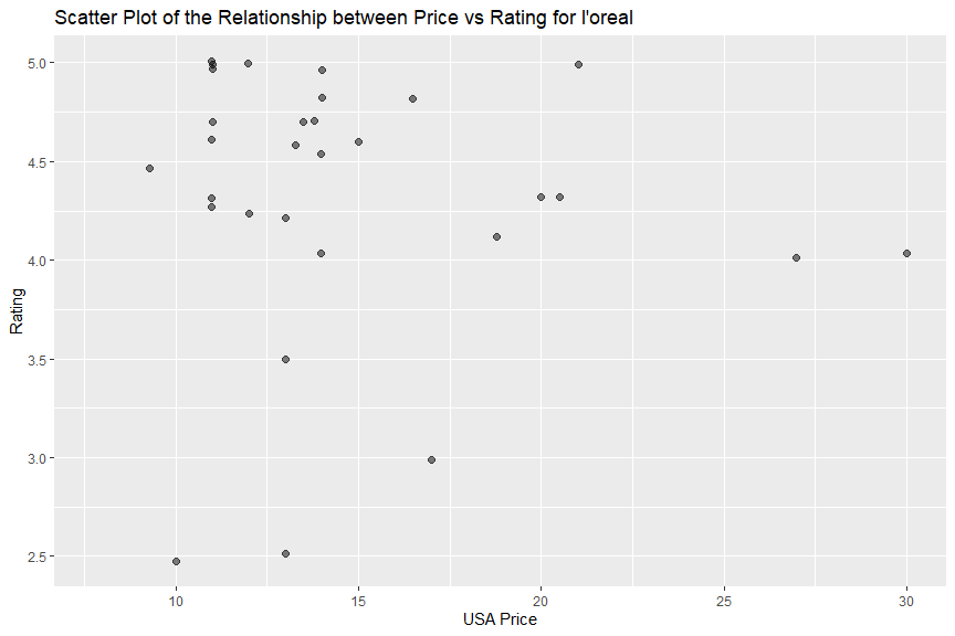
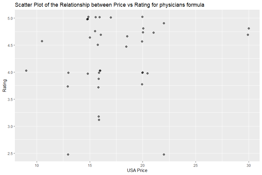
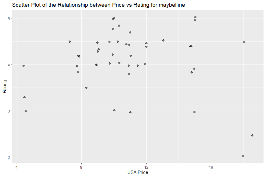
Scatter plots
Now I want to investigate whether there is any relationship between price and rating. I will still pick those 5 brand names that have most non-missing rating values.
I will put them in a list “a”, also write an anonymous function where
data frame will be filtered by the brand name input, then I am using the
ggplot function, mapping “rating” as y and “usd_price” as x. Later I
will add a geom_point layer to generate the corresponding scatter
plot. Finally I will use a lapply function to apply the anonymous
function to every element in the list “a”.
a <- list("covergirl", "l'oreal", "physicians formula", "maybelline", "revlon")
lapply(X=a, FUN = function(x) {
                       all_factor %>%
                       filter(Cosmetic_Brand == x) %>%
                       ggplot(aes(y = rating, x = usd_price)) +
                       geom_point( alpha = 0.5, size = 2, position = "jitter") +
              labs(y = "Rating", x="USA Price", title = paste0("Scatter Plot of the Relationship between Price vs Rating for ",x))})
## [[1]]
##
## [[2]]
##
## [[3]]
##
## [[4]]
##
## [[5]]
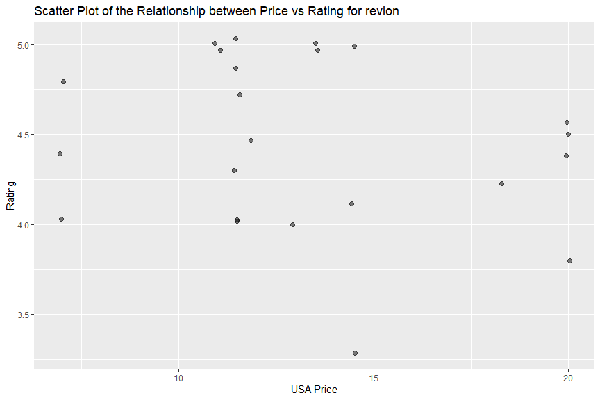
I did not observe clear relationship between price and rating from “covergirl”, “physicians formula”, “maybelline” or “revlon” data. There might be a week negative relationship between price and rating in “l’oreal”, which means its cheaper items had better ratings.
Second call
Next, I am interested in the brand “maybelline” which has many items in
this database with not great ratings. I am calling the API function
again and getting a subset data frame with only “maybelline” cosmetic
products, then converting its product type to factor by calling the
add_factor function.
# call the function and return a subset data frame with only maybelline cosmetic products
mbl <- pick_makeup(makeup_brand = "maybelline", makeup_type = NULL)

mbl_factor <- add_factor(mbl)
Second stacked bar graph
I will use gglot and geom_bar, assign cosmetic_type as x, also fill
colors based on different product type, to create a stacked bar graph
which presents item count for each product type.
q <- ggplot(data = mbl_factor, aes(x = Cosmetic_Type, fill = Cosmetic_Type))
  q + geom_bar(alpha = 0.7) +
  labs(x = "Cosmetic Type", y = "Item count", title = "Bar Plot of Item Count for Each Cosmetic Type of maybelline")
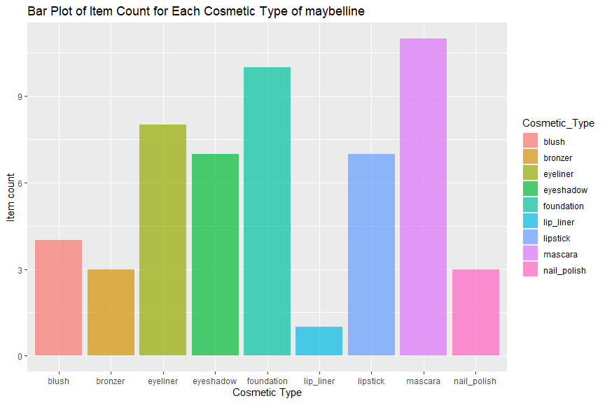
“maybelline” has items in all 9 product types, since this brand is famous for its mascara, the biggest product type is mascara and the smallest category is lip liner.
Rating summary by product type.
After removing records with missing rating, I am going to calculate the
rating mean, standard deviation, variance, median, Q1 and Q3 across
product types by using a group_by and a summarise function.
 mbl_factor %>%
            filter(is.na(rating) == FALSE) %>%
                   group_by(Cosmetic_Type) %>%
                   summarise(Mean = mean(rating),  Standard_Deviation = sd(rating),
                             Variance = var(rating), Median = median(rating),
                             q1 = quantile(rating, probs = 0.25),
                             q3 = quantile(rating, probs = 0.75))
## # A tibble: 9 × 7
##   Cosmetic_Type  Mean Standard_Deviation Variance Median    q1    q3
##   <fct>         <dbl>              <dbl>    <dbl>  <dbl> <dbl> <dbl>
## 1 blush          4.77              0.252   0.0633   4.8   4.65  4.9
## 2 bronzer        4.75              0.354   0.125    4.75  4.62  4.88
## 3 eyeliner       4.23              0.207   0.0427   4.25  4.05  4.38
## 4 eyeshadow      3.76              0.929   0.863    4     3.5   4.4
## 5 foundation     3.88              0.722   0.522    3.9   3.8   4.4
## 6 lip_liner      3.5              NA      NA        3.5   3.5   3.5
## 7 lipstick       4.4               0.849   0.72     4.8   4.2   5
## 8 mascara        4.16              0.241   0.0582   4.1   4     4.35
## 9 nail_polish    3.43              0.513   0.263    3.3   3.15  3.65
Surprisingly, the product type has the highest rating is blush instead of mascara. nail polish items have the lowest rating overall, eyeshadow’s rating has the widest range while eyeliner’s rating is more consistent.
A box plot
Lastly, let’s create a box plot and learn the price distribution across
product type. I will use a ggplot function and map price as y, product
type as x, also color each box according to their product type. Then I
am going to use a geom_boxplot function and add boxes onto the plot.
  b <- ggplot(data = mbl_factor, aes(y = usd_price, x = Cosmetic_Type, fill=Cosmetic_Type))
    b + geom_boxplot(adjust = 0.5, color="red", alpha=0.5) +
    labs(y = "Price", x="Product Type", title = "Box Plot of Price Center and Spread Across Product Type Groups")
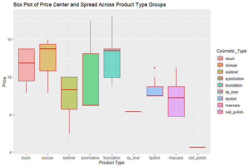
With lip liner and nail polish categories have either one item or one price, I won’t consider their distribution. The price distribution of blush and eyeliner categories are almost normal; bronzer, foundation and mascara are left skewed while eyeshadow and lipstick are right skewed. Brozer has the highest price overall and mascara has the lowest. Eyeshadow has the biggest price range and listick price is the narrowest with one outlier.
Wrap-up
In this vignette, I built several functions to interact with makeup
API’s endpoints. After data was returned, it went through some data
cleaning and manipulation steps to form an analysis-ready data frame.
The second half of this vignette focused on exploratory data analysis
(EDA). I used table, summarize and ggplot functions to generate
contingency table, numerical summaries of makeup price and rating, and
different plots for data visualization.
I found this vignette is actually handy for my future makeup shopping if they continually update the API with newly released items. I can search makeup products by brand and type, also compare their price and rating with the price and rating summaries from the same type products.
I did learn an interesting fact that some cheap items were rated much better than expensive ones, with this concept, I will save some money from cutting down high end products.
I hope this vignette will be known by more people especially girls, it could be helpful!